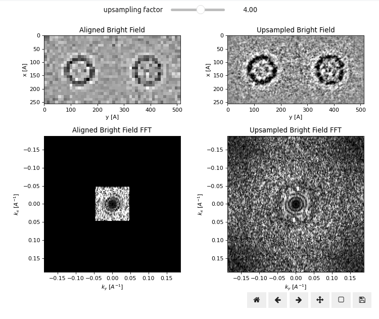
Upsampling of Aligned Bright Field
Subpixel Upsampling
As alluded to in previous sections, one of the strengths of tcBF-STEM is the fact that its resolution is not limited by the scan sampling, but rather controlled by the subpixel accuracy of the measured cross-correlation vector shifts, and ultimately limited by twice the convergence semi-angle Varnavides et al., 2023Yu et al., 2024.
In order to extract this additional resolution, we need to upsample our aligned virtual BF images stack using the following py4DSTEM snippet:
parallax = parallax.subpixel_alignment(
    kde_upsample_factor=4,
    plot_upsampled_BF_comparison=False,
    plot_upsampled_FFT_comparison=False,
)Note this does not simply perform Fourier upsampling, as can be seen from the additional Thon ring-like oscillations beyond the Nyquist scan-sampling limit. Instead, the sub-pixel accurate cross-correlation vector shifts are used to interpolating the virtual BF images stack using kernel density estimation (KDE) interpolation Ophus et al., 2016. Play around with the slider above to get a sense of how much additional resolution can be gained using KDE interpolation.
Aberration Correction
Notice how the aligned and upsampled virtual BF images we have investigated so far all have BF CTEM-like contrast. To account for this, and obtain contrast similar to that of the projected potential, we can use the estimated aberration coefficients to perform contrast transfer function (CTF) correction.
This correction can take many forms, but in py4DSTEM we choose to simply flip the sign of the even aberration coefficients and correct the asymmetry introduced by odd aberration coefficients using the following Fourier-space filter Lupini et al., 2016Varnavides et al., 2023
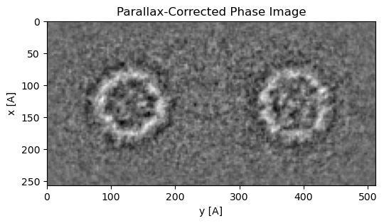
Figure 2 plots the aberration-corrected image following upsampling, which can be achieved using the following py4DSTEM snipppet:
parallax = parallax.aberration_correct(
    use_CTF_fit=True,
    figsize=(6,3),
    cmap='gray',
)- Yu, Y., Spoth, K. A., Colletta, M., Nguyen, K. X., Zeltmann, S. E., Zhang, X. S., Paraan, M., Kopylov, M., Dubbeldam, C., Serwas, D., & others. (2024). Dose-Efficient Cryo-Electron Microscopy for Thick Samples using Tilt-Corrected Scanning Transmission Electron Microscopy, Demonstrated on Cells and Single Particles. bioRxiv, 2024–04. https://doi.org/10.1101/2024.04.22.590491
- Ophus, C., Ciston, J., & Nelson, C. T. (2016). Correcting nonlinear drift distortion of scanning probe and scanning transmission electron microscopies from image pairs with orthogonal scan directions. Ultramicroscopy, 162, 1–9. https://doi.org/10.1016/j.ultramic.2015.12.002
- Lupini, A. R., Chi, M., & Jesse, S. (2016). Rapid aberration measurement with pixelated detectors. Journal of Microscopy, 263(1), 43–50. https://doi.org/10.1111/jmi.12372


