Tilt-Corrected Virtual BFs¶

The simulations shown in Virtual Bright-Field Images Stack used very fine sampling in both real-space (STEM probe positions) and Fourier-space (4D-STEM detector pixels). As we will see in Upsampling of Aligned Bright Field, one of the advantages of tcBF-STEM is that it drastically reduces both these sampling requirements, allowing us to collect more dose-efficient datasets Yu et al., 2024. In the remaining pages, we will work with a simulated 4D-STEM dataset using the same apoferritin sample, with the more realistic dimensions of $\left(R_x,R_y,Q_x,Q_y\right)=(24,48,128,128)$, i.e. $128 \times 128$ pixel diffraction patterns collected on a grid of $24 \times 48$ probe positions, with a spacing of $\sim 1$ nm and an electron dose of $100 \; e/\rm{\AA}^2$.

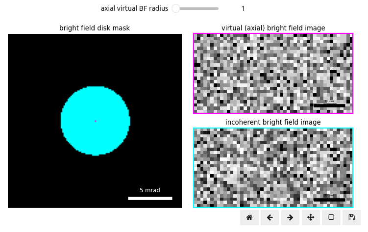
Figure 1 illustrates the BF disk on the left and a virtual BF image formed by the center-most pixel (right, magenta). Notice how much more noisy the virtual BF images look at realistic sampling conditions, as compared to Figure 1. We can bin the diffraction pattern further, to increase the signal-to-noise ratio (SNR) of the virtual BF images, by summing the intensity of nearby pixels together.

Source:py4DSTEM Parallax Masks Notebook

VBox(children=(IntSlider(value=1, description='axial virtual BF radius', max=26, min=1, style=SliderStyle(desc…

Play around with the slider below to increase the radius of the magenta pixels summed to produce the virtual BF image; you should find that while initially the SNR increases slightly, the faint protein signal gets blurred as we approach the radius of the BF disk to form what is referred to as an incoherent BF image (right, cyan). This is because, as we saw in Virtual Bright-Field Images Stack, the further away we get from the optical axis the greater the magnitude of the apparent shift of each virtual BF image and thus when averaged together introduces blurring. This is precisely the operation tcBF-STEM aims to “undo” Yu et al., 2024.

Iterative Alignment Bins¶

Put simply, what the tcBF-STEM algorithm attempts to do is to estimate the apparent image shifts of off-axis virtual BF images, align them with the optical axis, and sum their shifted intensity to boost the SNR, to bring all the virtual BF images in registry. In the open-source tcBF-STEM implementation in py4DSTEM Varnavides et al., 2023 this is achieved by employing a similarity measure called cross-correlation.

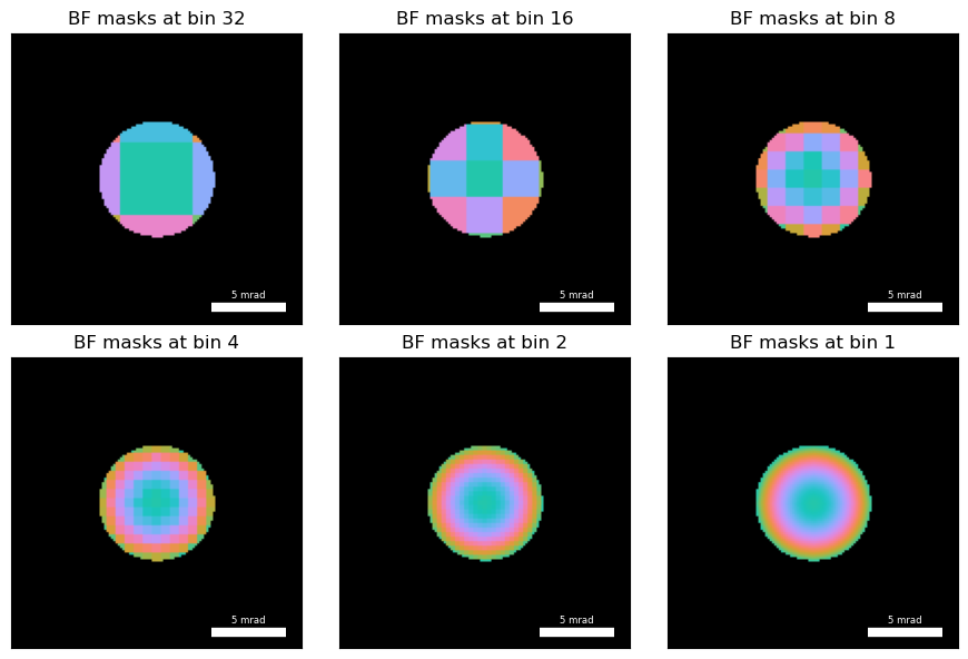
To ensure this procedure is robust against low SNR virtual BF images, we implement an iterative cross-correlation scheme. We estimate the cross-correlation vector field by binning the BF disk in decreasing smaller bin values and using the previous cross-correlation values as a starting guess for subsequent iterations. Figure 2 plots the the virtual BF masks used to compute the cross-correlation vector fields at each iteration.

Source:py4DSTEM Parallax Masks Notebook

Iterative Cross-Correlation¶

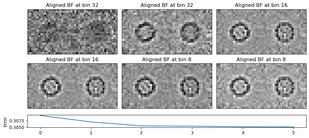
Despite the fact that the virtual BF images shown in Figure 1 have no discernible features the human eye can align to, iterative cross-correlation works remarkably well for this dataset. Note that in practice one often adds fiducial markers, such as gold nanoparticles, which produce strong amplitude contrast to ensure cross-correlation succeeds for very low SNR datasets Yu et al., 2024. Figure 3 illustrates the iterative alignment visually using the following snippet:

parallax = py4DSTEM.process.phase.Parallax(
    datacube=dataset, # py4DSTEM.DataCube
    energy = 300e3, # in eV
    object_padding_px=(8,8), # in pixels
).preprocess(
    edge_blend=4, # in pixels
    plot_average_bf=False,
).reconstruct(
    alignment_bin_values=[32,32,16,16,8,8],
    progress_bar=False,
    figsize=(10,4.5),
    cmap='gray',
)

Source:py4DSTEM Parallax Reconstruction Notebook

Notice how much crisper the aligned virtual BF image looks like as the iterative alignment proceeds, as-well as the monotonic decrease in the self-consistent error metric.

Cross-Correlation Shifts¶

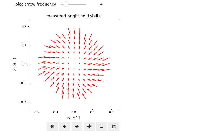
In addition to the aligned BF image, it is useful to inspect the cross-correlation vector field, i.e. the 2D cross-correlation vectors as a function of BF disk pixel position, directly. As we will see in Aberration Fitting, these hold a wealth of information pertaining to the microscope geometry and imaging conditions. Try playing around with the slider in Figure 4 to get a sense of the cross-correlation vector field.

Source:py4DSTEM Parallax Reconstruction Notebook

VBox(children=(IntSlider(value=4, description='plot arrow frequency', max=16, min=1, style=SliderStyle(descrip…