Nanocartography: Planning for success in analytical electron microscopy
Appendix
6.1Conversion to Cubic
In order to perform math on any crystal system it is first necessary to transform each system such that it can be described as a cubic cell. The simplest manner in which to accomplish this is to first constrain one of the new vectors onto the z-axis. For simplicity, and to match the convention that the beam axis is along the z-axis, c is chosen to align with the z-axis (Figure 6.1). As mentioned in the main body of the text, other equivalent starting choices could be made but they do not inhibit the overall conversion. The next step is to constrain the second of the new vectors in one plane. In this case, a is constrained to the xz plane, and then decomposed into the components of that plane using the angle β to the z-axis. Finally, the third vector is decomposed onto each of the x, y and z axes using the angles α, γ, and δ. The angle α is the angle from b to the z-axis. The angle γ is the angle between the vectors a and b. The last angle, δ, is an auxiliary quantity that is the angle between the projection of the b vector onto the xy plane and the y axis. Typically, a crystallographic system is specified with a, b, c, α, β, and γ. The auxiliary angle, δ, is then expressed in terms of these known quantities.
To understand how δ is related to the known quantities, a set of geometric objects is shown in Figure 6.2 to break down the calculation into smaller steps. Using the law of cosines on the triangle in the xy plane gives a relationship between the lengths of the three sides and the angle δ.
This has introduced another quantity, D, which is the length of the side of the triangle opposite the angle δ. Solving for δ yields:
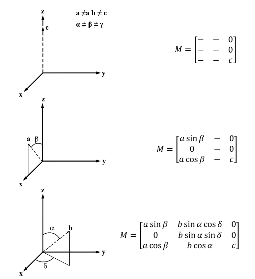
Figure 6.1:Schematics illustrating step-by-step derivation of the non-cubic to cubic conversion matrix.
To find the value of D, the Pythagorean Theorem is used on the right triangle with D as the base.
In this equation, G, is the side opposite the angle γ in the triangle which has legs a and b. The law of cosines is also applied here to find:
Eliminating to find and then substituting back into the equation for δ and simplifying the trigonometric functions yields a simplified expression:
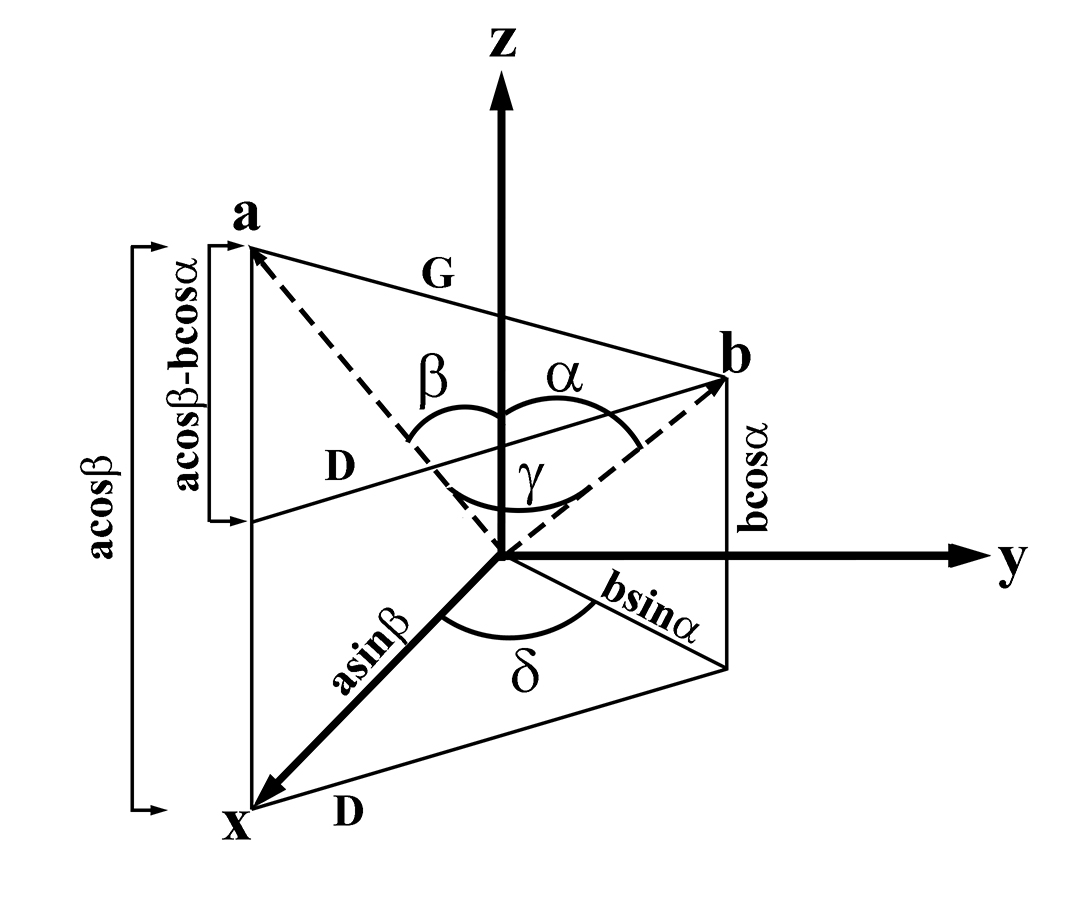
Figure 6.2:Schematic illustrating the calculation of the angle δ that accounts for non-orthogonal angles between axes in monoclinic and triclinic systems in the conversion matrix.
With the angle δ known, the full expression for the conversion matrix is what was presented above in the text as Eq. (6.6):
This matrix will convert a vector from a non-cubic system to a cubic system after matrix multiplication. The reverse process (going from cubic to a non-cubic system) is accomplished by multiplying by the inverse matrix. The inverse matrix for M is:
6.2Hexagonal to Cubic
Whereas (Figure 2.1) provided a simplistic example of the need to convert non-cubic systems to cubic before performing mathematical calculations, (Figure 6.3) illustrates a more complicated crystal system. A number of low index vectors in the hexagonal unit cell provided in (Figure 6.3), which are described in the native nomenclature and are invariable despite the c/a ratio (Figure 2.2). A schematic presentation of the cubic matrix conversion can be envisioned by placing a cube with the x and z axes commensurate with the hexagonal x and z axes and observing the traces of the vectors in the hexagonal system overlapping with the inserted cube. After a mental transcription of the vectors onto the cube, the hexagonal vectors can be removed, thereby leaving the vectors in the cubic cell. The positions of the vectors within the cube can then be observed. Mathematical operations, such as the angle between poles, can then be performed.
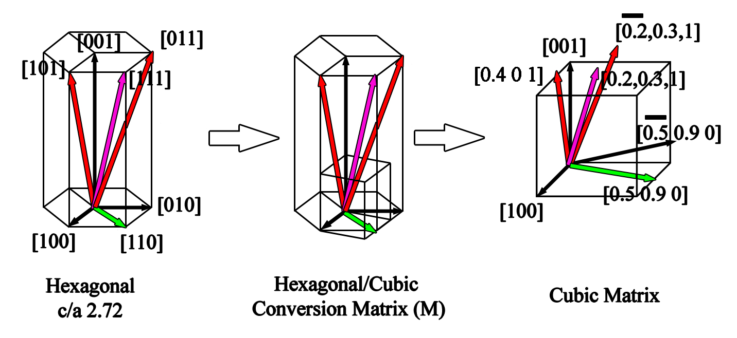
Figure 6.3:Illustration showing the conversion of a hexagonal matrix to cubic form.
6.3Rotation about an Arbitrary Axis
Rotations about the principal axes are simple to state, but are of limited use when considering general crystal orientations. Instead, it is useful to rotate about an arbitrary axis in space for any angle, not just rotation about one of the principal axes (Eqns. (2.6) to (2.11)). As previously stated, this rotation is not necessary to create useful tip/tilt maps, but it is necessary when comparing two crystals in a misorientation matrix. The misalignment that arises in the misorientation matrix as compared to the tip/tilt maps is that while the vector moves to the correct position in both derivations (e.g., the [111] to the [001]), the location of the unit vectors (i.e., [001], [100], and [010]) will vary depending on pathway. This will be derived subsequently, but is illustrated schematically in Figure 6.4.
The vector [uvw] is rotated to the [001] orientation about [xy0] through angle θ. The schematic details two pathways by which to achieve this rotation; path 1 which is about a single axis, and path 2 which is through two concurrent tilts about the additional unit vector axes (in this case x and y). In both cases the [111] vector is rotated to [001], but the location of the unit axes (as shown by the projection of a cube down the [111]) will differ by some angle (Δ) as compared to the rotation about the arbitrary axis. Note that the illustrated angle is exaggerated for effect, and is only approximately a few degrees. Depending on the order of the pathway, the angle (Δ) would also be different, hence providing two distinct projections of the unit vectors for misorientation calculations.
The example described above and illustrated in Figure 6.4 pertains directly to the formulation of a tip/tilt map for a double tilt stage (i.e., the rotation axis is always calculated normal to the [001] orientation), but a more general formulation of the tilt about an arbitrary axis needs be derived to account for non-crystallographic motions. Therefore, the full derivation is provided below.
To describe this general rotation, a sequence of steps can be used to decompose any rotation down into rotations about the principal axes. To accomplish this the desired axis of rotation needs to be rotated to coincide with any one of the principal axes through two rotations about the other axes (in the tip/tilt map calculation the z or probe axis is chosen). The desired rotation about the arbitrary axis is accomplished with the system aligned along a principal axis (e.g., ). Finally, the arbitrary axis is returned to its original location by performing the inverse of the first two rotations. For more details of this process, consult Cole, 2015.
The axis of rotation is a unit vector, and the desired angle of rotation about this axis is θ. Without loss of generality, the arbitrary axis will be rotated to the x-axis where the rotation by θ occurs. First, rotates into the x-y plane by rotating about the y-axis by an angle . This angle is computed by the requirement that the resulting vector, has no y-component. The angle which accomplishes this rotation is and can be found from the z-component (Figure 6.5).
In particular, since the y-component is unchanged and the magnitude of the vector is still 1, this intermediate vector can be written as . Next, the vector is rotated to point along the x-axis. This rotation is by an angle about the z-axis and the angle is determined by the requirement that the resulting vector should have no x-component. This angle is as can be seen by equating the y-component of the vector to 0.
These two angles move the vector to the x-axis, where it is rotated by an angle θ and then rotated back to the original position by rotating the negative of and . Combining all of these rotations into one yields the overall rotation matrix, :
In this equation, each rotation matrix is defined by the angle and the axis about which the rotation occurs. Note that the negative angle rotations are undoing the initial rotations to bring the vector to the x-axis and are the inverses of the first two rotations which can be found by taking the transpose of the and since for any rotation matrix, . If we express these matrices in terms of the matrices and simplify the trigonometric expressions in terms of the components of , then the matrix product is:
After matrix multiplication and simplification, recalling that the magnitude of is one , the full matrix for rotation of angle θ about an axis of rotation is:
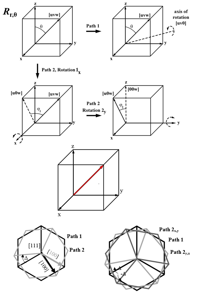
Figure 6.4:Direct rotation about an arbitrary axis as compared to two rotations about unit vector axes.
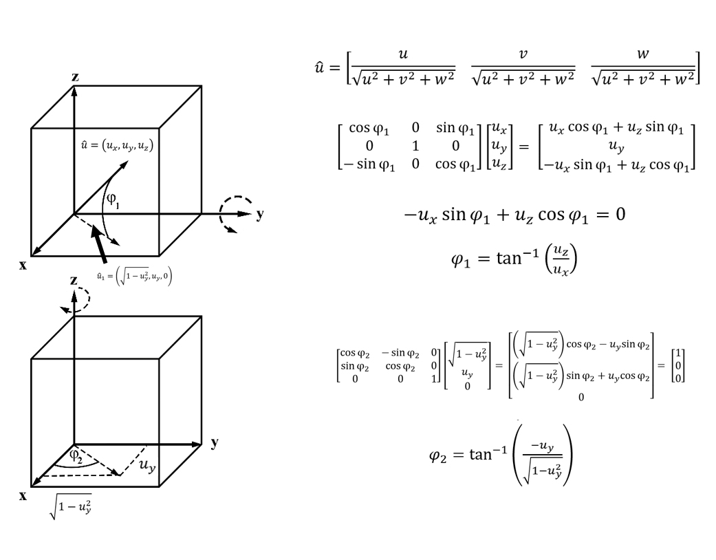
Figure 6.5:Schematics demonstrating the angles necessary to rotate around an arbitrary vector.
6.4Examples of Tip/Tilt Maps in Lower Symmetry Systems
As demonstrated in (Figure 2.7), tip tilt maps for cubic and hexagonal crystal systems can be procured in any number of orientations. The same can be done for other non-cubic systems such as tetragonal and orthorhombic (Figure 6.6a-c). In the [001] orientation a tetragonal crystal with a c:a ratio of 2 (as illustrated in Figure 6.6a,b) there are more accessible poles within an ~40° range as compared to the cubic form (i.e., Figure 2.7a). To demonstrate the asymmetry of the tetragonal system the [010] is plotted in Figure 6.6b. When the third unit axis vector is changed (i.e., orthorhombic), the larger asymmetry can be observed in (Figure 6.6)c. In order to best demonstrate how the tip/tilt maps can vary between a high symmetry system (e.g., cubic) and lower symmetry systems (e.g., monoclinic and triclinic) the [112] of the three systems is plotted in Figure 6.6d-f with the orientation of the [001] pole in each system ~15° from the α tilt axis. The various tilt positions of the [001] between the three systems as well as other surrounding poles highlights the large discrepancy when the unit axes and angles between axes varies. While each of these crystal system parameters were utilized from real crystals, it should be noted that the plotting of poles is in a general form to highlight the variability and does not fully represent whether each of the poles are expressed in those systems. Additionally, while the family of poles (e.g., the <112>) are plotted with the same format (e.g., blue dots) practically they are different families due to the variation in axes and angle between axes (e.g., the [112] is not in the same family of the [121] for a triclinic system).
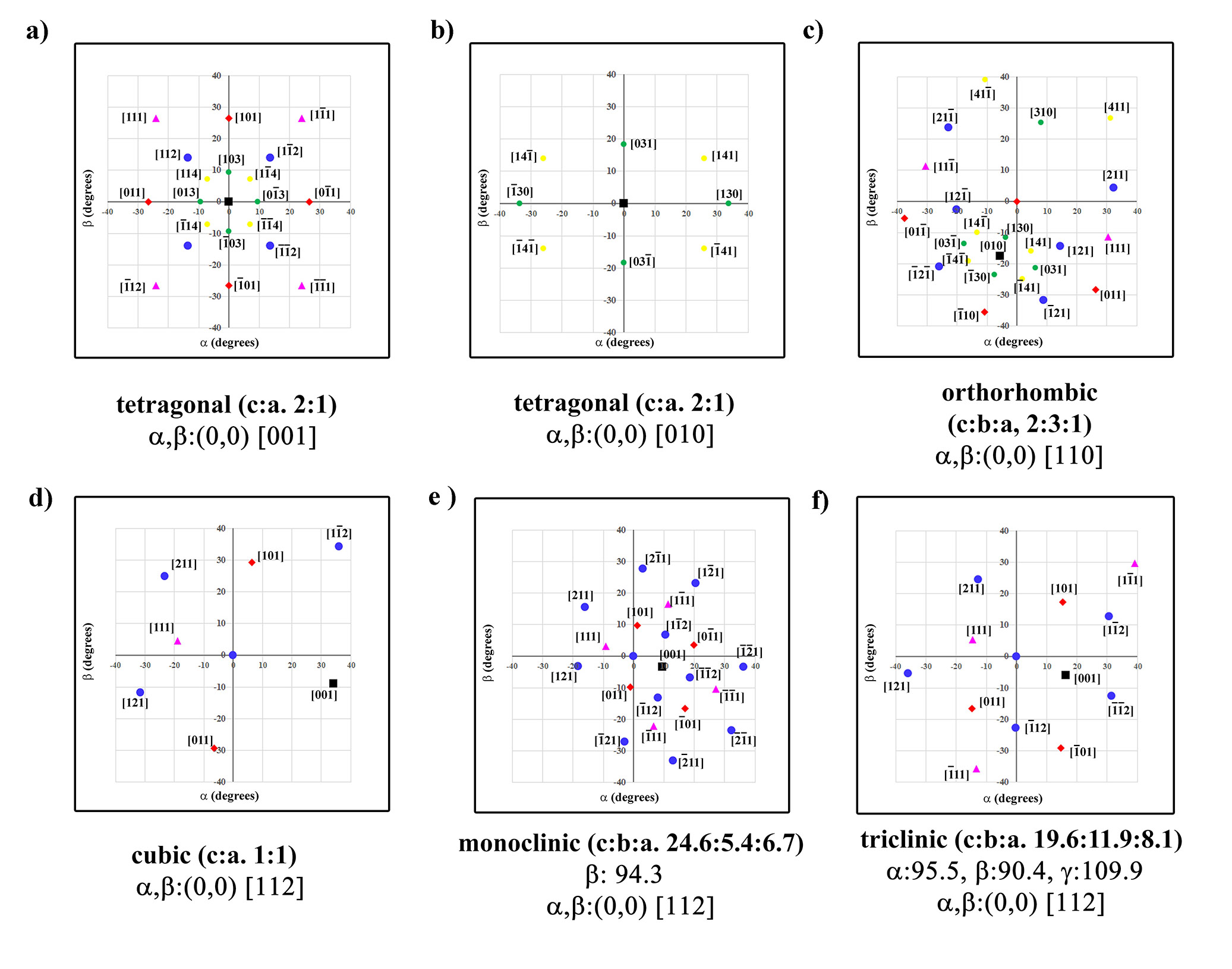
Figure 6.6:Tip/Tilt plots of various crystal systems.
6.5Plotting Kikuchi Bands
Plotting the traces of planes of atoms was accomplished by using the normal to the plane as an arbitrary axis by which to rotate any vector in the plane. This approach is not appropriate for tracing Kickuchi bands that are located at an angular distance equaling the Bragg angle from the trace of the plane of atoms. If these planes were to be plotted on a tip tilt map (Figure 6.7) it is unlikely that the precision of current double tilt stages would be able to discretely tilt to these conditions. In Figure 6.7 the [111] orientation of an FCC crystal is shown plotted on a tip tilt map with a corresponding Kikuchi pattern. The strong (4-40) bands shown in the Kikuchi pattern are the approximately the smallest d-spacings observed in all materials systems, and when plotted in the tip/tilt map it becomes apparent that all larger d-spacings would be bound within these lines (hence not within the precision of current double tilt holders). The projection of the large condenser aperture (~103 mrad) shown in the Kikuchi pattern is overlaid on the tip/tilt map for scale.
![Plot of tilt map for [111] FCC austenitic stainless steel in the [111] orientation with the {440} planes expressed (a) and a CBED pattern in the same orientation (b).](https://pub.curvenote.com/01919ca9-b718-74ab-9b96-74b341835a99/public/Figure A7-aeeb866cf4b663bf83ff0eb9c23b75fa.jpg)
Figure 6.7:Plot of tilt map for [111] FCC austenitic stainless steel in the [111] orientation with the {440} planes expressed (a) and a CBED pattern in the same orientation (b).
6.6Vector Equations to Matrix
The key to solving the system of equations for the coordinate vectors in Eqns. (3.19)-(3.21) is to rewrite them as vector equations for the elements of , and . Writing out all nine equations gives:
In this order, the patterns in these equations are not clear, so instead, they are grouped as Eqns. (6.13), (6.16), (6.19), Eqns. (6.14), (6.17), (6.20), and Eqns. Eqns. (6.15), (6.18), (6.21). These groupings yield:
In this grouping, these systems become much more recognizable as matrix equations:
In particular, the 3x3 matrices in each grouping are the same, which means that the same set of row operations will row reduce all of them simultaneously. As such, they are combined into a single augmented matrix that is Eqn. (3.22) in the text.
- Cole, I. R. (2015). Modelling CPV. https://repository.lboro.ac.uk/articles/thesis/Modelling_CPV/9523520

