Nanocartography: Planning for success in analytical electron microscopy
Mathematics of Navigation and Orientation in Three Dimensions
In order to most accurately utilize the TEM for crystallographic analysis it is first necessary to be able to express any crystal system as a geometrical concept. This approach serves to deconvolute the motion of a crystal as a solid object from the concepts of the crystal in reciprocal space, diffraction, or the physics of the electron beam interaction. These physics-based approaches are most often utilized in teaching materials science analysis using the TEM, but this adds additional complexity too early. By first treating any sample (which may or may not contain crystallographic material) as a solid three-dimensional object and how it can be manipulated using a double tilt stage, the additional concepts of diffraction and other electron beam interactions eventually becomes more intuitive.
Before any notion involving the addition of atomic positions to the discussion of crystallography and materials science, a general treatment of planes, plane normals, and other basic geometric constructs needs to be introduced and understood. This is necessary for a variety of reasons, most importantly of which is that it will provide a more solid foundation for both tilting throughout crystallographic space, as well as in general lay a solid groundwork for explaining Miller indices, Bravais lattices, and other such constructs. The extent of this discussion on geometry, while basic on some level, is necessary to further build upon the knowledge base of crystallographic analysis.
The simplest geometrical concept in crystallography is the cube due to its high level of symmetry and uniformity. All three unit vectors [u,v,w] can be oriented along the [x,y,z] axes, respectively, and any combination of vectors can be constructed. The mathematics of a cube are dependent upon each of the three axes being of equal length and mutually orthogonal to one another. The angle between any two vectors can be described by the dot product, and the normal of any two vectors can be calculated through the cross product.
2.1Unit Vectors – Real Space Map
The ability to travel through any crystal system is dependent upon understanding basic geometric principles of planes and directions. For example, the angle between the two cubic vectors [001] and [010] is 90°, between the [001] and the [011] is 45°, and lastly between the [001] and the [112] is 35.3°. These are all common low index (high symmetry poles) within any number of cubic crystals, and the understanding of how to move between these poles can be critical in proper microstructural analysis. Unit vectors are the fundamental descriptors of the cube and describe how to follow planes in the crystal to arrive at another location in the crystal. In this sense, the unit vectors function as the equivalent of roads on a map of a regularly laid out dense urban area.
Since there are six other crystallographic families by which atoms can be arranged, the importance of being able to travel between poles within each system is paramount to performing highly accurate crystallographic analysis. Similar vector notation can be used to describe any direction (i.e., vector) within each system (e.g., the [111] of a monoclinic crystal), yet the mathematical derivation of the angle between vectors or calculation of normal vectors is not as straight forward as applying the dot and cross-products due to either biases on the unit vectors or unit vectors not being orthogonal (or sometimes both depending on the crystal family). Figure 2.1 provides a simple example illustrating how a naïve analysis fails to accurately predict the measured angle owing to the bias of one axis. By stacking two cubes on top of one another to create a tetragonal unit cell, the z-axis can be described as having a bias (in Figure 2.1 is it biased by 2). In the schematic, the coordinate system is labeled in terms of what unit cell is being considered, either the biased cell or the cubic cell, and hence biased vectors in the tetragonal reference (or native format) are listed as [0,0,1] and [1,1,1], whereas in in the cubic reference they would be [0,0,1] and [1,1,2]. Calculating the angle between these vectors in both the biased and the cubic coordinates (through the dot product), it can be shown that the answers differ by 19.4°, with the calculations for the biased system being incorrect (as it will be shown later on in the paper, 54.7° is a common angle in the cubic system because it is the angle between the [001] and [111] poles). Only when the native vectors are converted to the cubic form is the correct answer, 35.3º, obtained. A demonstration of this conversion in a more complex, hexagonal system is provide in Figure 6.3.
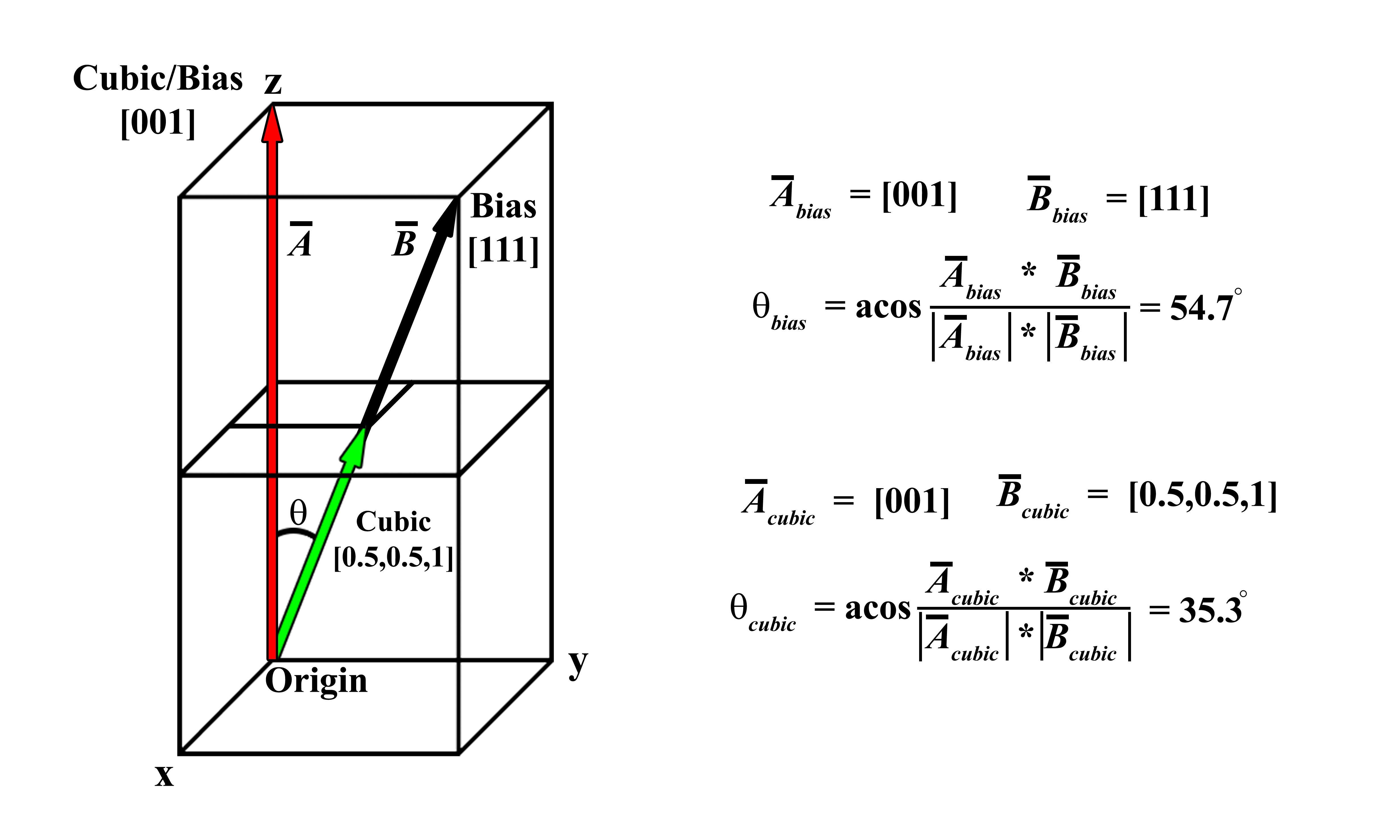
Figure 2.1:Schematic illustrating how a bias on one of the axes (e.g., a tetragonal system) does not provide the correct angle between vectors. The bias of the z-axis being doubled incorrectly predicts the angle between the vectors. Note the positions are being listed in parenthesis and do not denote crystallographic planes.
The importance of vector nomenclature as compared to the vector calculations can be further elucidated by comparing a single crystal system (e.g., hexagonal) where the ratio of the unit vectors are varied (Figure 2.2). Native vectors for hexagonal crystals with c/a ratios of 2.72 and 1.63 are described in the identical manner owing to the fact they are the same crystal system, but when converted to the cubic form the vectors are now noticeably different. Since the vectors within the basal plane (e.g., [100] and [110]) are not affected by the change in c/a ratio, the angle between the vectors does not change, but comparing the angle between the [001] and the [111] it can quickly be demonstrated that in the cubic system the [111] vector becomes [0.2 0.3 1] and [0.3 0.5 1] for the hexagonal crystals with c/a ratios of 2.72 and 1.63, respectively. Performing the dot product on the respective vectors illustrates how the angle between the [001] and [111] vectors can change by ~10.4° with a change ~66.8% c/a ratio (note that for ease of comparison to the cubic system, the three index notation is used for the hexagonal system). The ability to derive a conversion matrix for any given crystal system is necessary to perform these operations.
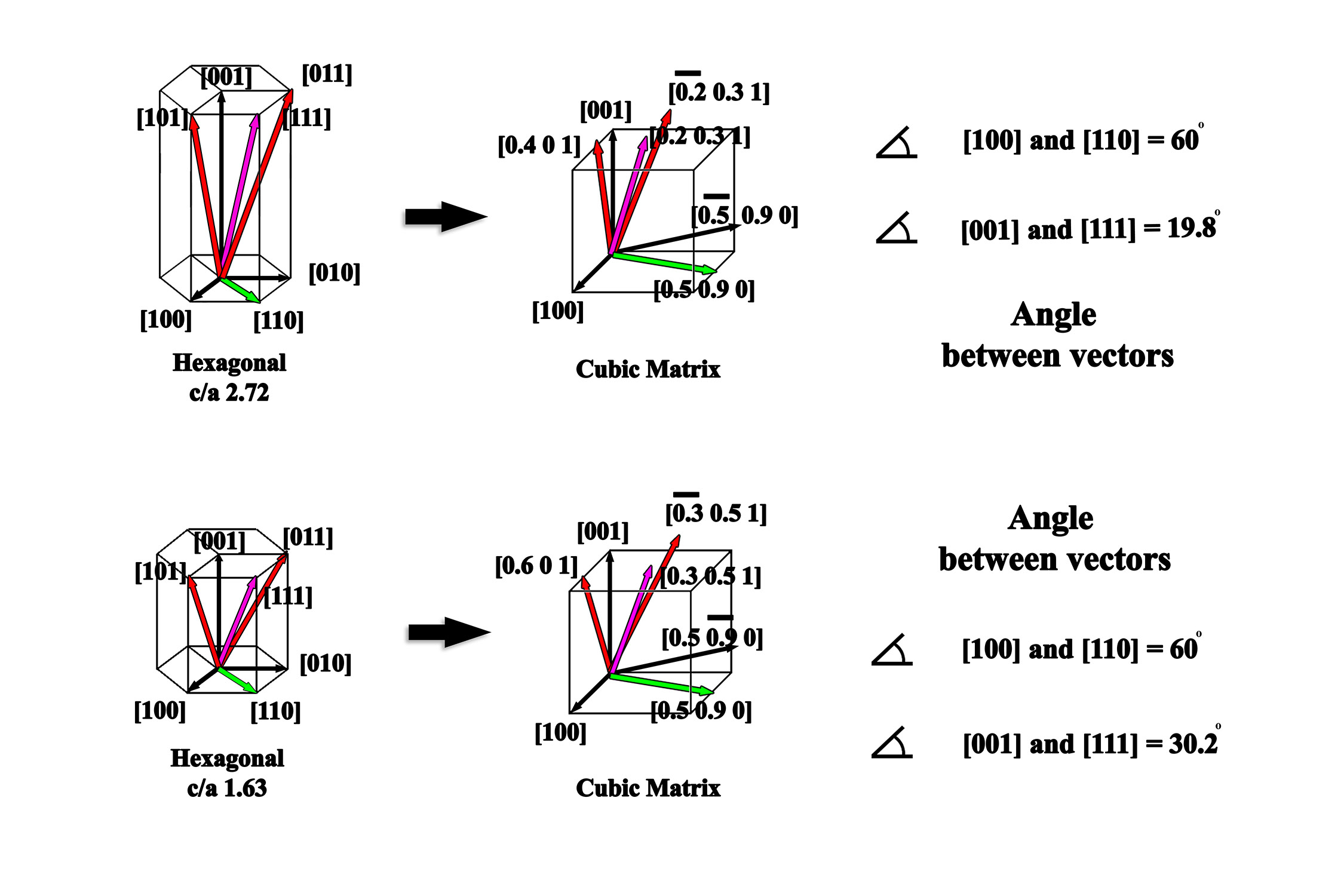
Figure 2.2:Comparison of vector nomenclature in the native hexagonal system as compared to the cubic formulation.
In order to travel about any of the other seven crystal systems (e.g., between poles) is it necessary to understand how to convert the axial and non-orthogonal biases into cubic/Cartesian form (note that for ease of comparison in the field of materials science, the term cubic will be utilized in the remainder of the paper). For the other orthogonal systems, the only consideration is the length of the bias, whereas for the remaining non-orthogonal systems there are angular dependencies on the axes in addition to length bias. In the overwhelming majority of materials science and electron microscopy textbooks, similar calculations are performed and presented as conversion formulas for each system. Again, these formulas are usually confined to describing angle between planes, and do not explicitly describe how to calculate the plane normals. This is typically performed because of the need to calculate the angle between diffracting planes and overlooks how to calculate the normals, which are needed to predict how to travel around each crystal system. The foundation for deriving all relevant crystallographic properties become available through the understanding of the pure geometric conversion of each crystallographic system to the cubic system. As an alternative formulation of this problem, these types of crystallographic computations can be calculated through the use of the metric tensor, as detailed by De Graef and McHenry De Graef & McHenry, 2012 . While both approaches are mathematically correct, this work has chosen to preserve the intuitive sense of angles and distance in the cubic system, albeit with the requirement of a conversion matrix for non-cubic systems that will be described next.
The conversion of any non-cubic system (abc) to that of a cubic one (xyz) uses a conversion matrix (M) Eq. (2.1). A schematic of illustrating the two systems is shown in Figure 2.3 along with the conversion matrix with the full derivation of this conversion matrix is provided in the Appendix (Conversion to cubic in Figure 6.1 and Figure 6.2). Later, when discussing the microscope setup in more detail, the z-axis will be chosen to align with the electron beam. Consequently, we have chosen to align the c axis of the crystal that is to be converted with the z-axis for conceptual simplicity. This is certainly not the only choice, and the following derivations could be followed with a different convention, such as the one used by International Tables of Crystallography Aroyo, 2016. However, the essence of the method is unchanged regardless of the specific convention used.
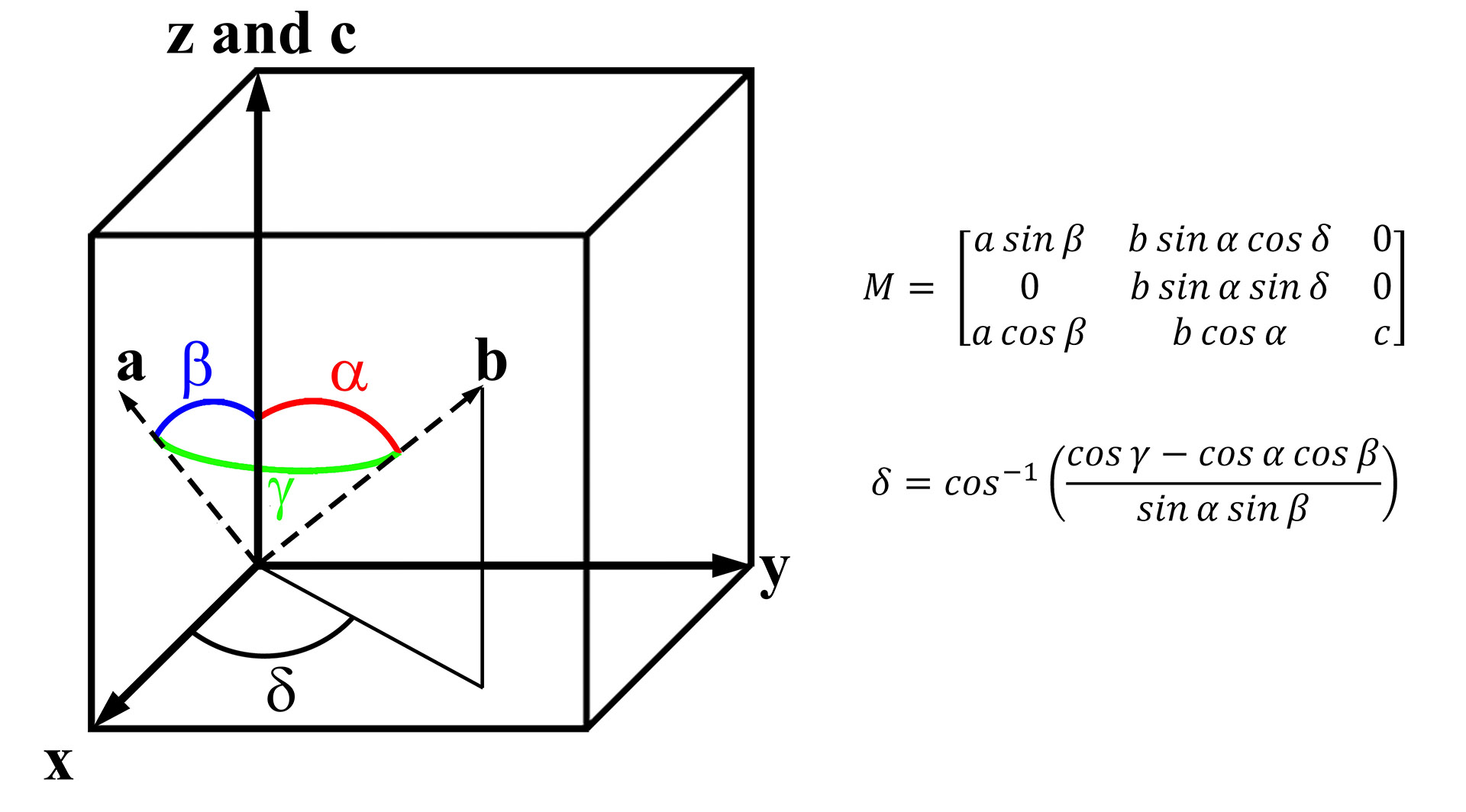
Figure 2.3:Schematic illustrating how to convert any non-cubic vector coordinate system into a cubic system and the conversion matrix (M).
The derivation of the conversion matrix, Eq. (2.1), which includes the angle δ, Eq. (2.2), can be calculated from the principal axis angles (α,β,γ). The conversion matrix operates by setting one axis in the system to be converted equal to one axis in the cubic system (e.g., the c axis is first set commensurate with the z-axis in Figure 2.3). This is then followed by setting a second axis in the system to be converted and binding it within two of the axes in the cubic system (e.g., the a axis is restricted to the xz plane). The a axis can then be decomposed into the x and z components (i.e., there is no y component) through sine and cosine functions of the angle β, respectively. Lastly, the final axis of the system to be converted to the cubic system (in this case b to y) must be decomposed into all three axes of the cubic system (a full explanation is provided in the Appendix). The introduction of a fourth angle, delta (δ) Eq. (2.2) must be employed to account for the less symmetric crystals such as the monoclinic and triclinic where the angle γ is not 90°. The conversion of any crystallographic vector in any crystal system can then be calculated by multiplying the vector by the conversion matrix Eq. (2.3).
As an example, the [111] vector in the tetragonal unit cell as exhibited in Figure 2.1, when converted to the cubic system can be described as a [0.5 0.5 1] (or [112]) vector, which is 35.3° from the [001] in the tetragonal system (the [001] converted by Eq. (2.3) remains the [001]). These equations can then be utilized for any of the seven crystal systems for which the angle between vectors (i.e., poles) can be calculated with the understanding that the vectors are described in their native form but are calculated in the cubic form (an example of a hexagonal system conversion if presented in Figure 6.3). As such, all the remaining operations will be performed on cubic systems with the understanding that it can be generalized to any crystal system using the appropriate conversion matrix, or its inverse.
While it has been described as the ability to travel throughout a crystal, a more elegant manner in which to describe these conversions is to envision all possible vectors within a cube. The “movement” around the system is the pathway between vectors. These pathways will eventually be considered traces of planes, and hence how to travel along these specific planes. The notion of predicting the location of all poles is important because it will subsequently be demonstrated that when considering electron beam interactions the structure factor will simply act as a filter to determine which of these poles are ultimately expressed for any given crystal.
2.2Stereographic Projections – Rotation Maps
The stereographic projection is most often utilized by microscopists to navigate and understand crystalline sample orientations (Figure 2.4). As illustrated in Figure 2.4a the stereographic projection is a calculation of the relative location of all vectors for a given crystal provided a specific normal orientation (e.g., the [001] in Figure 2.4a). In the keeping with the context of this paper, the utilization of the stereographic projection keeps with the notion of first understanding the motion of the sample and crystal in real space and does not consider reciprocal space (i.e., Kikuchi bands).
There are different conventions for stereographic projections, typically whether the center of the sphere or the bottom of the sphere should be located at the origin, but they all contain the same fundamental information. Returning to the map analogy, this is analogous to different map projections (e.g., Mercator vs. Robinson) Lapon et al., 2020. In this formulation, the sphere has a radius of 1 and is centered at the origin. To compute the location of these poles, consider a cubic crystal with one corner at the origin and [100] along the x-axis, [010] along the y-axis, and [001] along the z-axis. The intersection of the vector normal to a plane of atoms with the sphere and the top of the sphere define a line, as seen in Figure 2.4a. The intersection of the line with the plane z = 0 defines the planar coordinates of the projection. Mathematically, if a pole is at [uvw], then it is normalized to have unit length Eq. (2.4) to find its intersection with the unit sphere. When observed in two dimensions (Figure 2.4b) the relative position of each vector and the trace between the vectors can be derived Eq. (2.5).
The line connecting the top of the sphere [0, 0, 1] and this point will intersect the z = 0 plane at
![Geometric stereographic projection (in the [001]
direction) in three dimensions (a) and the corresponding two-dimensional
stereographic projection (b).](https://pub.curvenote.com/01919ca9-b718-74ab-9b96-74b341835a99/public/Figure 4-cbd21574c71630ac54b25c27d99c7b0f.jpg)
Figure 2.4:Geometric stereographic projection (in the [001] direction) in three dimensions (a) and the corresponding two-dimensional stereographic projection (b).
It is important to note that when describing non-cubic pole figures, the native description of each pole is utilized such that when analyzing and reporting data there is an objective reference. Equally important to introduce here is the notion of the freedom of rotation within a pole figure. The stereographic projection can be considered as viewing a cube down a specific orientation and then determining how far and in which direction to rotate the crystal to align to another pole. The use of stereographic projections is useful when examining three-dimensional ball and stick models in computer programs designed to visualize orientations of crystals. Most programs will allow for the input of specific vectors, and it is worth pointing out that when a non-cubic system is visualized the poles/vectors are listed in a native coordinate system, but the mathematics are calculated by converting to a cubic system as shown above in Eqs. (2.1)-(2.3). In the electron microscope, the use of a double tilt stage adds an additional conversion that must be applied in order to travel throughout any crystal due to the limitation of the degrees of freedom.
2.3Double Tilt Holder Coordinates – Tip/Tilt Map
As has been demonstrated by numerous other researchers, understanding the utilization of a double tilt stage in the analysis of solid materials and crystals is extremely important for accurate and reliable data collection Cautaerts et al., 2018Liu, 1994Liu, 1995Qing, 1989Qing et al., 1989. While this has been reported on numerous occasions, the following derivation will be presented in a manner by which to convert three-dimensional rotations in simple geometric constructs to the double tilt stage and then demonstrate how this relates to reciprocal space and the physics of electron beam interactions. Given that different manufacturers utilize different terminology, as a matter of convention, the tilts of a double tilt stage will be denoted as α, β, and will be equivalent to X, Y tilts, respectively.
While stereographic projections are useful, they do not directly translate to the sample in the microscope due to the restrictions of the tip/tilt stage on which the sample is mounted. To accurately describe the position in terms of a double tilt holder, a tip/tilt map must be derived. This map plots the poles and planes of the crystal in terms of the tip and tilt coordinates of the double tilt holder and allows the prediction of all allowable poles within a specific orientation of a given sample. It should be noted that the derivations for converting from a stereographic projection to a tip/tilt map is reversible, and hence the tilt coordinates could and have been utilized overlaid on top of stereographic projections.
The importance of the motion of the double tilt holder as compared to a stereographic projection is the freedom of rotation considered for both. Figure 2.5 provides the stereographic projection and tip/tilt map of a cube in the [001] orientation. In a stereographic projection the crystal can be rotated freely, hence oblique plane traces are straight (when emanating from the origin), whereas in the double tilt holder oblique plane traces will be curved (Figure 2.5). This curvature, as will be illustrated in the subsequent derivations, is a result of the β tilt axis changing as a function of the α tilt, and hence S-type curves are generated in a tip/tilt map. A trace of a single plane in the tip/tilt map (red line, Figure 2.5b) has been overlaid on the stereographic projection (Figure 2.5a) to illustrate the difference. Additionally, when the position of three vector types (<103>, <114>, and <112>) in the tip/tilt map are transposed onto a stereographic projection, and it can be observed that the farther from the [001] orientation the larger the misorientation (e.g., the [114] vectors are located nearly in the same position, but the [112] are visibly misoriented).
This is also the exact reason why obliquely oriented g-vectors collected at high tilt angles in a double tilt stage (e.g., α,β:-25,-25) will rotate slightly in plane with relation to those collected at α,β:0,0. This is shown in the attached movie in Figure 2.5c. Therefore, it is necessary to be able to convert a stereographic projection to a tip/tilt map for any given crystal system. This can be achieved through rotation matrices.
2.4Rotation Matrices
While rudimentary, in terms of the overall development of the stage motion the fundamental mathematical operation being utilized is the rotation about a single axis. This rotation is typically described as a rotation about any of the primary axes (x,y,z), but more generally, any orientation can be described through successive rotations about these three axes (Eqs. (2.6)-(2.8)). The rotation about any primary axis will be defined by the right-hand rule so that rotation matrices about the x-, y-, or z-axis through an angle θ are given by, respectively:
Note that for these rotation matrices they are defined by the angle of rotation and the axis about which the rotation occurs. In addition to rotations about a single axis (i.e., proper rotations), there are also improper rotations (i.e., reflections about an axis) that describe mirroring about a single axis (Eqns. (2.9)-(2.11)). These can be illustrated in matrix form:
These are the basic building blocks upon which more general rotations can be built and will be referred to continuously when performing matrix operations to rotate the crystal and orient the sample. Whether rotating along a specific interface, tilting from pole to pole, or re-loading a sample and converting prior tilt conditions, these six formulae will be the basis set. In the following derivation of the tip/tilt map the utilization of diffraction and crystallographic terminology will be utilized but only as a frame of reference and not in terms of the electron beam interaction (i.e., traces of planes and not g vectors or Kikuchi bands).
In practice, the manner in which a microscopist interacts with a crystalline sample is at the most basic level through diffraction spots or Kikuchi lines. While the principal knowledge of what these optical markers represent goes to a fundamental understanding of electron beam interactions with samples, at the very core of electron microscopy as an observational tool, the understanding of these as fiduciary markers for roadmaps provides the basis for nanocartography. That is to say, regardless of whether one understands the physics of why a zone axis (ZA) appears, the observation and acknowledgement of a zone axis as a combination of a series of geometrically oriented Kikuchi lines (or order diffraction patterns) is necessary to be utilized as a map.
These traces along with the knowledge of the double tilt stage can be used to solve unknown crystals and also predict the motion of interfaces. In the current context of deriving a tip/tilt map, the knowledge of a specific pole type is assumed for the purpose of ease of explanation. This assumption is made as an initial means to connect vector motion to crystallographic analysis. For instance, as shown in Figure 2.6a, the six fold symmetry of the [111] in an FCC steel is presented along with a tilt position (e.g., α,β : 5,10) in which this orientation was discovered in the microscope (note that the correct nomenclature should be <111> as it is a description of the family of poles, but for ease of explanation a single vector will be used).
This “known pole” provides the first bit of knowledge as to a global position with respect to the remainder of the crystal. This could also be a diffraction pattern of the [111] pole, but for ease of understanding a convergent beam electron diffraction pattern (CBED) is presented. The in plane orientation of the crystal is described by the angle () that can be used to describe the rotation of the crystal about the known pole. As will be subsequently described, the angle can be used to freely rotate the crystal (Figure 2.6b-d), or it can be assigned as a specific fiducial marker (such as the (1-10) Kikuchi line) with known relation to the calibration of the α tilt axis. The tilt positions observed (e.g., α,β : 5,10) can then be used to mentally envision the relationship of the found ZA to the tilt stage (Figure 2.6b, where the stage has been returned to α,β:0,0). This crystal rotation can best be considered by illustrating a vector in a cube (e.g., [111] in Figure 2.6) in both the standard projection (Figure 2.6c) and a projection normal to the vector (Figure 2.6d), and the being the relative rotation by which the entire cube rotates. Again, while the CBED pattern of the [111] is presented, it is only used to orient the practical aspect of the microscope to developing a tip/tilt map. From these initial data, the tip/tilt map can be derived as follows.
There are two orientations that will be considered: the orientation of the crystal with respect to the probe, and the stage with respect to the probe. The probe will be considered an objective frame of reference oriented at [001]. The orientation of the sample can be described for any crystallographic orientation within the sample, whether a single grain or the orientation of two crystals across a boundary. Figure 2.6b shows an observed pole (red and blue) for two grains, of which the unit vectors for each crystal in black. The knowledge of the location of the observed poles and the unit vectors will be important for obtaining the most information from a sample (e.g., the local misorienation between two grains).
In order to create a tip/tilt map, the known vector will be rotated through a sequence of rotations to align it with the [001] probe orientation, subsequently rotated with respect to the crystal orientation () using , and finally the stage will be tilted from the probe position to the found conditions (observed tilts) (Figure 2.6e-g). The known pole will be utilized to derive the entire rotation matrix representing the crystal orientation, and subsequently any other possible vector can then be plotted accordingly through that matrix.
The mathematical derivations of the full rotation matrix are divided into three steps. The first step, , represents the orientation of the sample with respect to the holder as it is inserted into the microscope (Figure 2.6e). The second step, , aligns the mathematical description of the crystal with the one found in the microscope (i.e., α,β of the known pole and rotation of the crystal ), but as shown in Figure 2.6f it does not consider the tilt conditions. The last step, , puts the pole at the location corresponding to the known α,β coordinates observed (Figure 2.6g). Taken together, the multiplication of these matrices yields an overall rotation matrix, that contains all the orientation information about the crystal as it is situated in the microscope. Again, it is important to note that the only necessary functions are combinations of the rotations provided in Eqns. 2.6-2.11.
One of the major advantages of these derivations with regards to previous calculations on stage motion Cautaerts et al., 2018Klinger & Jäger, 2015Liu, 1994Liu, 1995Qing, 1989Qing et al., 1989 is in the power of creating a sample map which can be utilized in subsequent analyses whether on the same microscope or at other institutions. This allows for rapid re-analysis of samples without losing previous crystallographic orientation data. Three terms are required that will allow the sample to be reloaded into any microscope in any orientation and convert any previously recorded tilt coordinates to the current sample loading. The application of these matrices account for the sample being flipped in the holder either horizontally ( , Eq. (2.12)) or vertically ( , Eq. (2.13)) to the long axis of the holder, and as well if the sample had been rotated in-plane by any angle ( , Eq. (2.14)) (Figure 2.6e).
The combination of these sample reloading matrices can be combined into one matrix as shown in Eq. (2.15). Note, the angle is measured and recorded through a global fiduciary marker (e.g., the surface of a FIB lamella) during each analysis. In the instance where there is no horizontal or vertical flip (i.e., the initial analysis of the sample), then these matrices are be replaced with the identity matrix (i.e., no rotation is applied).
Once the sample has been loaded into the microscope and a known pole has been identified, the mathematical model of the orientation of the crystal is matched to the orientation of the sample. The first step in developing this correspondence is rotating a known vector (e.g., the [111]) to the probe direction [001] through a rotation matrix ( Figure 2.6f). It is important to note that this is setting the orientation of the crystal to the probe, and thus the tilt conditions of the stage are not considered. For ease of explanation, the use of vector terminology instead of crystallographic designations (such as ZA or crystal pole) will be utilized to describe the motion of a crystal in a stage.
The rotation of this vector to the probe direction can be achieved through a number of pathways (e.g., combination of rotation matrices), but the most direct is a rotation about an arbitrary axis by an angle (θ) (Figure 2.6f). As the vector will always be rotated to the [001] direction to be aligned with the probe, the axis of rotation will always lie in the xy plane and will take the form of [uv0] because it is calculated through the cross-product of the known vector and [001] (see Figure 6.4). It should be noted that this is special to this case, and a more general formulation needs to be derived for a general operation. This will be subsequently utilized to describe the trace of planes.
The known pole need first be normalized to create a unit vector. The dot product is used to compute the angle required to move this unit vector in the direction of the pole from its standard orientation (i.e., at in Cartesian coordinates):
The axis of rotation is determined from the cross product of the normalized known pole and the beam direction:
For these specific axes of rotation that have no z-component (i.e., in the derivation of tip/tilt maps), and the general result simplifies to (where rx and ry are derived from Eq. (2.17), and θ from Eq. (2.16)):
The mathematical derivation of the rotation matrix () of an angle θ about an arbitrary axis is presented in full in the Appendix (Figure 6.4 and Figure 6.5). As an aside, it should be noted that with respect to crystallographic tip/tilt maps, the rotation about an arbitrary axis is not necessary. Two rotations (and subsequent inverse rotations) can be utilized that will accomplish the same rotation, but in subsequent utilization of these derivations for calculation of the local misorientation angle and axis between two adjacent grains there will arise a misalignment depending on the order of rotation. This is discussed in further detail in the Appendix section surrounding (Figure 6.5).
As previously described, in order to orient the crystal with respect to the known pole (Figure 2.6a) an additional rotation is required. Since the crystal has been rotated to the z-axis, the rotation of the crystal through the angle about the z-axis (Eq. (2.8), ) will rotate the crystal about the known pole. Combining the rotation of the known pole to, and about, the z-axis provides the full definition of .
Whereas the rotation of the known vector to the probe direction was accomplished through a direct rotation from one position to another, the majority of double tilt stages do not operate in this manner and are performed through a two-step process with one axis beholden to the other. As can be illustrated in Figure 6.4 , the order of rotation in a two-step process can affect the outcome of the final position, and hence order of tilt is a necessary consideration. The rotation of any vector to the final tip/tilt location α/β is accomplished by multiplication by followed by . This combination is called the rotation matrix of the stage Eq. (2.20) where the tilt conditions for the known vector α,β are substituted in to Eqs. (2.6) and (2.7), respectively.
The order of these rotations is important in the sense that the tip/tilt stage rotations are not interchangeable. Since the rotation of one holder axis (α in this case) does not change the axis of rotation of the second tilt (β), the first rotation is about the α axis. This allows the use of an active rotation framework presented above without difficulty where the axes are considered fixed. While a passive rotation formulation would be logically equivalent, mixing the two would lead to incorrect results. The most striking example of the fact that the order of rotation matters is that the tip/tilt diagram is not symmetric in the location of poles as previously illustrated in the stereographic projection as compared to the tip/tilt map (Figure 2.5).
To summarize this set of operations, the action of all these rotations in concert can be summarized in the total rotation matrix:
Finally, it is important to understand that this matrix operation provides the Cartesian coordinates of the poles (i.e., a 3x1 matrix), and hence these final values must be converted to α/β coordinates. An intuitive way to understand this conversion is to consider the rotation of a vector from (0, 0, 1) to (X, Y, Z) in Cartesian coordinates, where . This conversion amounts to solving for the angles α/β that satisfy:
After multiplying and solving the individual equations, the final tilt angles are:
The X,Y,Z terms are not the vector describing the known vector or any starting vectors, but the final converted vectors through (e.g., if the known vector was [111], XYZ would not necessarily be defined by [111]). Note that these can be expressed in terms of other trigonometric functions that are equivalent mathematically, but it is most convenient to use the inverse tangent function in practice because it accepts signed inputs for both its inputs which allows angles to range anywhere from –π to π. This removes the requirement to adjust the quadrant of α/β explicitly. Once α/β have been computed for every pole of interest, then the poles can be plotted as a function of α/β to create the tip/tilt diagram detailed above. A demonstration of stage movement is shown in Figure 2.6 h and i that shows simple sample tilt in beta (Figure 2.6h) as well as with a representative BCC Si phase ball and stick model to illustrate how the crystal would rotate with the stage (Figure 2.6i).
To better demonstrate this, a discussion of plotting of various poles and tilt conditions for both cubic and hexagonal systems is provided. Cubic vectors [001] and [111] oriented at the (α,β:0,0) condition with a variety of other vectors are shown (Figure 2.7a and b, respectively). The asymmetry of the double tilt stage movement presented in Figure 2.5 and again in Figure 2.7a becomes apparent, with the [112] not being located at equal α,β conditions when the (-110) is oriented 45° to the α tilt axis (it is observed at (α,β:24.1,26.6)). This is due to the β tilt dependency on the initial α tilt. Subsequent analysis of directions between poles will elucidate this in greater detail.
The vectors presented in these representations are arbitrarily based on what would represent lower index crystallographic poles, and as it were, any vector could be plotted. The plot of the [110] (Figure 2.7c) at tilts (α,β:10,20) is shown to illustrate how a discovered pole at a non α,β:0,0 tilt condition would appear to provide a more representative scenario of what would be observed in the microscope. In this orientation the <111>, <100>, and <112> low index poles are in the field of view. Additionally, the bounds of the tilt stage limits can be overlaid upon these maps to further discriminate the allowable poles within a specific grain.
In order to demonstrate how the conversion of non-cubic systems are handled, hexagonal plots are presented (Figure 2.7d-e). These figures illustrate a hexagonal system with a c/a ratio of 1.63 in both the basal [001] and primary prism [210] orientations at tilts (α,β:0,0). In the basal [001] orientation the [111] pyramidal poles are plotted, and in the primary prism [210] the secondary prism [100] are observed at (30,0) and (-30,0). As a demonstration of how the vector projections change with a change in c/a ratio, the [001] projection at (α,β:0,0) for a hexagonal system with a c/a ratio of 2.72 is presented in Figure 2.7f. The elongation of the c axis draws the [111] type vectors closer towards the (0,0) tilt position and as well the [1-11] type vectors are now within the applicable 40° tilt range. This change in c/a ratio can also be observed in Figure 2.2. Additionally, with the change in c/a ratio it is also noted that the angle between the primary and secondary prism poles do not change because they are orthogonal to the c axis, and hence are unaffected. The reader is guided to the online code (insert inline documentation here) to create basic tip/tilt maps for any system at their leisure.
Systems that are more complex could also be illustrated (see Supplemental Figure 6.6 for examples), but it should again be mentioned that a) that while the vectors are described in their native format, the math is done in a cubic form, and b) any vector possible may be plotted because these are vector representations. The plots in Figure 2.7 represent generic crystals/maps for the given crystal system (i.e., cubic and hexagonal), and do not represent real crystals. The presentation of these maps are solely meant to illustrate the tilt parameters for solid objects in real space. This sets the basis for the derivation of crystals in reciprocal space to explain the travel of planes of atoms within a crystal.
![Tip/Tilt plots of the cubic system with [001],[111] at
the α,β:0,0 (a and b, respectively) and the [110] at α,β:20,10 (c),
and the hexagonal unit cell (d-f) with c/a ratios of 1.63 (d,e) and 2.72
(f) with either the [001] (d,f) or [100] (e) at α,β:0,0](https://pub.curvenote.com/01919ca9-b718-74ab-9b96-74b341835a99/public/Figure 7-18a8a8466c219d5a10854fdeedd04974.jpg)
Figure 2.7:Tip/Tilt plots of the cubic system with [001],[111] at the α,β:0,0 (a and b, respectively) and the [110] at α,β:20,10 (c), and the hexagonal unit cell (d-f) with c/a ratios of 1.63 (d,e) and 2.72 (f) with either the [001] (d,f) or [100] (e) at α,β:0,0
2.5Calculation of Planes in a Tip Tilt Map
The development of a tip/tilt map for any given crystal system provides a manner in which to predict the tilt motion of any possible vector within each system. These tip/tilt maps are most relevant to stereographic projections or pole figures that indicate the motion between poles within a freely rotating system. In order to make a more complete comparison, it is necessary to add a description of the travel between poles. This will also facilitate the transition from real space to reciprocal space when discussing crystallographic planes. The understanding of the real space calculations is not only imperative for crystallographic motion, but as will be demonstrated, the identical formulations can be utilized to define the pathways of other physical constructs, such as interfaces and free surfaces within the sample.
This discussion must be prefaced with the explicit understanding of these motions with respect to crystallographic terminology as to not further confound the already difficult task of differentiating real space and reciprocal space. Kikuchi lines are a representation of inelastic scattering that diffracts from crystallographic planes at the Bragg angle, and while the derivation and presence of allowed diffracting planes will be considered in subsequent sections, their introduction here is used as a manner by which to suggest that just as plotted poles can be represented as in both stereographic projections and tip/tilt maps, so too can the travel between any of these poles be calculated or mapped. Again, the presentation of these will be discussed in simple geometric terms and then later elaborated upon in terms of crystallography and electron beam interaction.
Concerning plotting actual Kikuchi lines as compared to plotting the tilt coordinates between various poles, a standard convention must be adopted. While Kikuchi lines are formed in pairs corresponding to both the positive and negative g vectors, within the accuracy of any double tilt stage given possible errors such as motor backlash and machining tolerance it is more convenient to plot a single set of directions for the trace of any given plane whose vector has been normalized (i.e., the normal of the (222) can be described as [111]). This is not to say that the mathematics could not be derived for the exact tilt coordinates for each specific allowed plane for any crystal, but in terms of practical analysis, the normalized vector for each family will be considered. Figure 6.7 illustrates a tilt map for an FCC austenitic stainless steel (unit cell ~3.86 Å) oriented in the [111] orientation with the {440} planes expressed, and a CBED pattern in the same orientation. These Kikuchi bands represent a major plane that would be expected to be oriented farther out within k-space, and still the tilt angle is ~1°. Therefore, the proposed method is a conversion of a stereographic projection into tip/tilt space more than it is a conversion of a crystalline stereographic projection.
To plot the trace of any given crystallographic plane, especially for non-cubic systems, the normal to the plane must first be calculated and then subsequently converted to the cubic form. This formulation is modulated by the crystal structure and structure factor that is discussed in detail in the subsequent section. Only the cubic form will be discussed herein since the description of the normal to the plane is the same as the plane itself. The trace of the plane can be considered as the plot of all possible vectors within the plane, and therefore a rotation matrix with the plane normal substituting for the arbitrary axis of rotation is necessary (see Figure 2.8). As will be shown, this rotation matrix is nearly identical to the rotation about an arbitrary axis () derived in with the caveat that a more generic derivation can be developed that is not required to tilt to the beam direction.
The rotation matrix can be calculated by first determining any normal vector (green arrows Figure 2.8b) to the plane normal (red arrow Figure 2.8a,b), where this vector lies in the desired crystallographic plane. This truly arbitrary rotation matrix is found by evaluating (6.12) with the arbitrary axis of rotation being the plane normal and the angle of rotation becoming the desired step size of the line to be plotted. A set of vectors is created by applying the rotation matrix to one of the poles repeatedly until it returns to its original location (in the case of 1-degree steps this will yield 360 total vectors). Because these vectors are in standard orientation, they must be rotated as the poles were above through the multiplication of . This will yield the Cartesian vector sequence which then is required to be converted to α/β coordinates using Eqns. 2.23-2.24. Computing these sequences for various low index planes of interest yields in each system the complete tip/tilt diagram that can be seen in Figure 2.9. Variation of crystal parameters, starting poles, tilt conditions, and stage limits are allowable. Whereas the normals can be described by the Miller indices in the cubic system, for the hexagonal planes the plane normal first needed to be calculated, subsequently converted to cubic, and then plotted. As has been previously mentioned (Figure 2.5), due to the motion of the double tilt stage the traces of the planes can exhibit S-curves and are not always straight. This motion is exactly how the planes of atoms within the microscope behave across the entire tilt space, and the reason why g-vectors in diffraction patterns collected at different ZA can appear to rotate in relation to one another. The calculation of the vector normal, or g-vector, to these hexagonal planes will be discussed in the next section.
![Tip/tilt maps of cubic and hexagonal crystals oriented at
with the [001] and [001] (a and b, respectively) at the (α,β:0,0)
positions.](https://pub.curvenote.com/01919ca9-b718-74ab-9b96-74b341835a99/public/Figure 9-c8e0843dd599972aea2b094d74baf792.jpg)
Figure 2.9:Tip/tilt maps of cubic and hexagonal crystals oriented at with the [001] and [001] (a and b, respectively) at the (α,β:0,0) positions.
These derivations combine many different aspects of previously published research but have been presented in the manner of simple geometric considerations for the purpose of deconvoluting the physical nature of electron microscopy samples from the physics of electron beam interaction. The ability to understand the motion of and samples within a double tilt stage is imperative, and then subsequently being able to connect that knowledge to the physics of electron beam interaction can elevate any research whether the crystal structure of the desired sample is known, or more importantly if it is not. As an example, the description of interface motion can be modeled after the motion of the trace of crystallographic planes, thus allowing for the microscopist to orient crystals and physical objects such as grain boundaries or surfaces.
2.6Reciprocal Lattice Vectors – Reciprocal Space Maps
The study of nanoscale electron beam interactions with solid materials (most importantly crystals) in the electron microscope has been a hallmark of the technique and has drastically expanded any number of scientific fields. The previous sections treated samples only as geometric objects in order to more easily orient the reader as to how vector and matrix mathematics can be utilized to travel through a sample. This knowledge is extremely useful even when the material is unknown. When crystalline orientations are known, this information can then be mapped onto the strict geometrical derivations previously discussed. While there are countless topics (over a century’s worth of research) surrounding electron beam interactions with crystals, this paper will concentrate solely on the structure factor due to its role in which planes of atoms (and hence poles) are exhibited for any given crystal. It is beyond the scope of the work to go beyond this, and with respects to the topic of nanocartography it would not be relevant.
With the considerations of any crystal as a simple geometric construct or unit cell (e.g., a cube or hexagon), the introduction of the atomic packing within these cells will dictate when a crystallographic plane will be expressed via diffraction. By first illustrating how any infinite number of planes or vectors can be plotted and manipulated, the discussion of which planes can be observed for a given crystallographic sample becomes clearer than first introducing reciprocal space and then demonstrating how it can be manipulated through three-dimensional space.
The description of the travel between poles has been previously demonstrated, and these derivations can also be considered to travel along a specific plane within that body. In the derivation, the tilt coordinates for every normal to a desired pole were calculated, hence forming the directions along the plane. In order to relate these derivations to electron beam diffraction it is necessary to convert the crystal to reciprocal space and determine the normal of any plane.
It should be noted that this is slightly different than how this topic is typically presented with the angle between planes being derived for each crystallographic system in addition to the d-spacing within a crystal Carter et al., 1996. While this is important for the analysis of diffraction patterns, it does not account for calculating the normal for any plane within any crystal. It is well known (and is often the basis of materials science education) that the description of the normal to a plane of atoms in a cubic crystal is the same description as the plane (i.e., [uvw] = (hkl)). While the mathematical analysis of the angle between poles is straightforward, more often than not when the discussion of non-cubic systems is broached the introduction of the angle between planes is introduced without further explanation (e.g., hexagonal systems).
The conversion of any pole within any crystal was demonstrated in Eqs. (2.1)-(2.3), but this was considered in the realm of real space. Crystallographic analysis with regards to diffraction is always considered in reciprocal space, and hence the derivation of the normal to any crystallographic plane is necessary. The unit vectors in reciprocal space must be derived by first considering the unit vectors in real space (i.e., the [100], [010] and [001]) (Eqs. (2.25)-(2.27)). For a cubic system this simply becomes [a00], [0b0], and [00c] because the orthogonal nature of the crystal precludes any of the trigonometric operators in the conversion matrix from being anything other than 1 or 0. As shown in Figure 2.1, introducing the unit cell bias of a tetragonal system where a equals b but does not equal c, the unit vectors are still the similar description as the cubic system because of the orthogonality of α, β, and γ, save for the magnitude of c. When these three angles are not mutually orthogonal, the length of the unit vectors is a combination of the lengths of the unit cell and angles describing the cell as calculated by the conversion matrix Eq. (2.1) multiplied by the unit axes vectors:
Once the unit vectors in real space have been derived, the unit vectors in reciprocal space are then formulated by crossing the opposite unit vectors in real space and then dividing by the volume of the cell Eq.(2.28) to gain the lengths of the unit vectors in reciprocal space (Eqs. (2.29)-(2.31)). The volume of any parallelepiped can be calculated by taking the cross product of two of the unit vectors dotted by the third. In condensed form it appears in Eq. (2.28).
The cubic unit cell can then be calculated by combining the reciprocal unit vectors (Eqs. (2.29)-(2.31)) into a 3x3 matrix which can then be used to calculate the g-vector Eq. (2.32) in the cubic form for any plane. Derivation of the inverse of this matrix multiplied by a given native normal will provide the plane associated with that pole. It should be noted that while the native description of the plane of atoms (hkl) (e.g., (111) tetragonal c/a =2) is utilized for this calculation, the resultant g-vector is in cubic form. As previously discussed, the cubic form is necessary to plot planes of atoms in a tip/tilt map, as well calculate the angle between planes Eq. (2.33) and determine the d-spacing of plane (Eq. (2.34). This distance between any plane is then the length of the normal vector in cubic form. It should be stressed that when plotting or representing the planes, the nomenclature for the native planes are still used. The description of the native normals can also be calculated for demonstration purposes (Eqs. (2.35) and (2.36) by multiplying the cubic description of the normal by the inverse of the conversion matrix (M-1). The initial example provided in this article (Figure 2.1) utilized a tetragonal cell with a c/a ratio of 2 to demonstrate the calculation of the angle between two vectors. A similar schematic illustrated in Figure 2.10 for a similar tetragonal crystal where the plane normals for (111) and (212) planes are shown both in their native and cubic forms. Whereas in (Figure 2.1) the [111] native normal was listed, it does not describe the normal for the (111) plane. Figure 2.10 illustrates that the native normal for the (111) is actually the [441] (which converts to [221] in the cubic form).
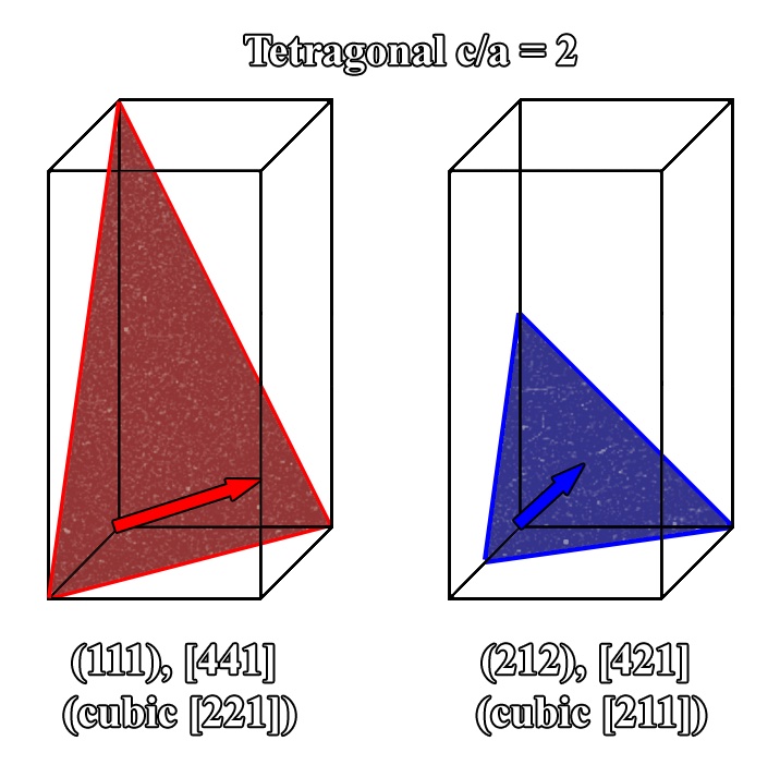
Figure 2.10:Schematic of two planes in a tetragonal crystal showing the relationship of the plane normal in the native and cubic form.
2.7Structure Factor – Tip/Tilt Filter
The organization of this research was designed to begin in real space, define how to take any solid geometrical object such as a cube or hexagonal prism, and then rotate that object. Next, these Cartesian coordinates were converted to double tilt stage coordinates and it was demonstrated how confining the degrees of freedom required a second set of coordinates. The conversion of real space into reciprocal space was then examined in order to best introduce the idea of how the description of real crystals could be mapped on top of the tip/tilt calculations. Just as the real space calculations considered any pole/vector normal possible, so did the description of crystals in reciprocal space provide any possible set of poles/planes/vectors based on the simple geometry of the crystal. The last portion of this discussion goes further into examining real crystals and how they interact with an electron beam, more specifically the structure factor and how it acts as a simple filtering function for the aforementioned calculations. That is to say, all possible combinations of vectors, crystal systems, planes, and normals were provided, and the structure factor provides a way to determine which of all of those combinations are exhibited in any crystal.
As noted prior, countless other electron beam interactions relate to diffraction and scattering contrast that could be discussed. In the context of this paper the structure factor is most relevant, and even then only a cursory explanation will be provided to illustrate the power of understanding the connections between the real space and reciprocal space in regards to materials analysis. More detailed descriptions of the physics of these interactions can be found in any number of electron microscopy texts Carter et al., 1996De Graef & McHenry, 2012Thomas, 1962.
The structure factor as it pertains to this discussion is a means to determine which planes of atoms within any given crystal will diffract. In terms of diffraction and the TEM, tallying the combinations of allowable diffracted planes can then be used to create a list of allowable expressed poles. The use of these lists can then be utilized to create tip/tilt maps by which to travel throughout any crystal given provided recognition of specific planes and poles is possible (Figure 2.11).
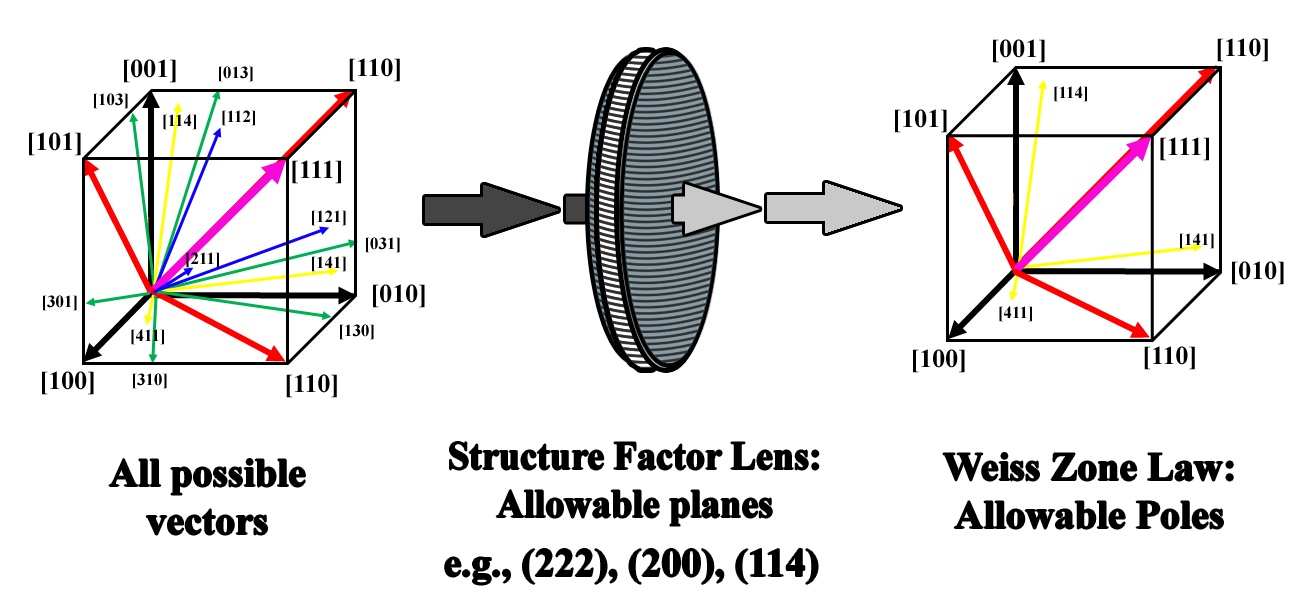
Figure 2.11:Schematic showing the use of the structure factor as a filter to determine which of the infinite number of vectors in real space are expressed in reciprocal space (ZA).
Whereas the conversion of crystal systems in real space into reciprocal space considered all possible combinations within each structure, the physics of real crystals are defined by the arrangement and packing of any number of atoms within the unit cells of the 7 different crystal systems. The complexity and variation of this packing is evidenced by the 230 possible space groups within these systems, not to mention the increased complexity of quasi-crystals and quasi-crystal approximants. In order to distinguish which planes within each crystal will diffract, the position and scattering power of each atom is considered. The equation for the structure factor Eq. (2.37) is provided below for any given plane of atoms described by (hkl), and depending on whether the solution is nonzero or zero dictates whether or not the plane will diffract, respectively. This can be further expanded to account for more complex crystals with any number of atoms each at any position within the unit cell. Note that since the atomic positions of each atom are used, there need not be any conversion from non-cubic systems.
where fj is the scattering factor of the j-th atom, xj,yj, zj are the atomic coordinates, and hkl defines a reciprocal lattice point corresponding to real space planes defined by the Miller indices. After a list of allowable planes is calculated, the trace of each of these planes could be plotted in either a stereographic projection or tip/tilt map, of which they would automatically intersect at the possible poles expressed for each crystal. Moreover, a combination of allowable poles could be derived by determining only those planes that satisfy the Weiss Zone law Eq. (2.38). Depending on the definition of applicable poles (i.e., which poles exhibited appreciable Bragg diffraction spots), the positions of those poles could be calculated using Eq. (2.38) and plotted.
These tip/tilt maps of well-defined crystals are only a small part of what can be accomplished utilizing the information contained herein.
- De Graef, M., & McHenry, M. E. (2012). Structure of Materials: an Introduction to Crystallography, Diffraction and Symmetry. https://doi.org/10.1017/CBO9781139051637
- Aroyo, M. (2016). International Tables for Crystallography. International Union of Crystallography. https://doi.org/10.1107/97809553602060000001
- Lapon, L., De Maeyer, P., De Wit, B., Dupont, L., Vanhaeren, N., & Ooms, K. (2020). The Influence of Web Maps and Education on Adolescents’ Global-scale Cognitive Map. The Cartographic Journal, 1–14. https://doi.org/10.1080/00087041.2019.1660512
- Cautaerts, N., Delville, R., & Schryvers, D. (2018). ALPHABETA: a dedicated open‐source tool for calculating TEM stage tilt angles. Journal of Microscopy, 273. https://doi.org/10.1111/JMI.12774
- Liu, Q. (1994). A simple method for determining orientation and misorientation of the cubic crystal specimen. Journal of Applied Crystallography, 27(4), 755–761. https://doi.org/10.1107/S0021889894002062
- Liu, Q. (1995). A simple and rapid method for determining orientations and misorientations of crystalline specimens in TEM. Ultramicroscopy, 60(1), 81–89. https://doi.org/10.1016/0304-3991(95)00049-7
- Qing, L. (1989). An equation to determine the practical tilt angle of a double-tilt specimen holder and its application to transmission electron microscopy. Micron and Microscopica Acta, 20, 261–264. https://doi.org/10.1016/0739-6260(89)90059-2
- Qing, L., Qing-Chang, M., & Bande, H. (1989). Calculation of tilt angles for crystal specimen orientation adjustment using double-tilt and tilt-rotate holders. Micron and Microscopica Acta, 20, 255–259. https://doi.org/10.1016/0739-6260(89)90058-0
- Klinger, M., & Jäger, A. (2015). Crystallographic Tool Box (CrysTBox): automated tools for transmission electron microscopists and crystallographers. Journal of Applied Crystallography, 48, 2012–2018. https://doi.org/10.1107/S1600576715017252
- Carter, B., Carter, D., & Williams, D. (1996). Transmission Electron Microscopy: A Textbook for Materials Science. Diffraction. II. Springer. https://doi.org/10.1007/978-0-387-76501-3
- Thomas, G. (1962). Transmission electron microscopy of metals. Wiley. https://doi.org/10.1107/S0365110X6200287X

